VoltLab
Open projectVoltLab began as a small interaction: place a few components, connect wires, and see what happens. I kept that idea, but the product grew around a stricter set of requirements. The workspace needed to feel natural on a desktop, remain usable from the keyboard, show the same circuit in schematic or realistic form, and explain the simulation instead of hiding it behind a number.
The goal was not to reproduce every industrial device model. It was to build a fast, educational simulator where the circuit on the canvas, the values in the inspector, and the solver’s explanation all come from the same model.
What you can do
- Build and edit circuits from a component palette.
- Connect stable component ports with wires, route points, and explicit junctions.
- Move, rotate, flip, group-select, copy, paste, duplicate, and delete circuit elements.
- Draw, split, reshape, and remove wire routes.
- View the same circuit as a schematic or in a more realistic presentation.
- Run, pause, step, stop, and reset a simulation.
- Display electron-flow, conventional-current, or no-flow overlays.
- Inspect voltage, current, power, and component-specific readouts.
- Change model inputs such as voltage, resistance, capacitance, inductance, switch state, and LED limits.
- Save and load circuit documents as JSON.
- Undo and redo document edits with keyboard shortcuts.
- Zoom, pan, snap to a configurable grid, fit the circuit to the viewport, and format layouts automatically.
- Review solver diagnostics and failure-lab examples instead of receiving unexplained numerical errors.
The model behind the canvas
VoltLab treats electrical connectivity as data. The canvas is a view of that data.
| Part of the model | What it means |
|---|---|
| Components | Electrical parts with named, stable ports, properties, defaults, and readouts |
| Wires | Connections between ports or junctions, independent of canvas coordinates |
| Junctions | Explicit graph entities that make branching connections unambiguous |
| Waypoints and routes | Visual geometry attached to a connection, not the definition of the circuit |
| Documents | JSON data that can be saved, loaded, imported, and exported |
That separation lets a user move a component without changing the circuit underneath. Selection, grouping, copy and paste, automatic layout, and undo and redo operate on the editor while the solver continues to work from the same graph.
The equations behind the simulation
The canvas is for people. The solver works from the circuit graph and the electrical relationships represented by each component. The implementation is educational, but it is still grounded in the laws a learner expects to see:
| Principle | How it appears in VoltLab |
|---|---|
| Kirchhoff’s Current Law | At every node, the signed currents add up to zero, ΣI = 0. Explicit wires and junctions tell the solver which component ports share that node, so current cannot disappear at a branch. |
| Kirchhoff’s Voltage Law | Around a closed loop, voltage rises and drops balance, ΣV = 0. Node potentials and source branch constraints are solved together, preserving the voltage relationships around the loop. |
| Ohm’s law | A resistor is stamped as a conductance, G = 1/R, and its current is read from I = V/R. |
| Capacitors | A capacitor uses a backward-Euler companion model with G = C/Δt and a current source based on its previous voltage. |
| Inductors | An inductor uses R_eq = L/Δt and its previous current to represent the transient relationship at the current time step. |
| Diodes and LEDs | A piecewise companion model changes its conductance around the forward drop and is rebuilt during nonlinear iterations. |
This is why explicit junctions matter. They are not only drawing details. They define the nodes where Kirchhoff’s current law is evaluated.
How a solve proceeds
- The topology analyzer validates the graph and separates independent circuit islands.
- Connected ports are mapped to nodes. Voltage-source and inductor branches receive extra unknowns so the matrix can represent their voltage constraints and currents.
- Each component stamps its contribution into the system through conductances, current sources, or voltage-source branches.
- The linear system is solved with pivoting and a residual check. VoltLab rejects bad pivots instead of silently regularizing a singular circuit into a believable-looking answer.
- Nonlinear devices are re-stamped and solved again until the largest change in the unknown values is below the convergence tolerance or the iteration limit is reached.
- For a transient simulation, each visible update is split into bounded time steps. That keeps an AC waveform, a capacitor charge curve, or an inductor current from jumping over the behavior the learner is meant to see.
The defaults are kept in one solver policy so the numerical decisions are visible and testable:
| Parameter | Default | Purpose |
|---|---|---|
| Base time step | 0.05 s | The normal interval used by the transient model |
| AC samples per cycle | 24 | Keeps the fastest AC waveform from being sampled too coarsely |
| Maximum transient steps | 512 | Prevents one large playback jump from taking over the interface |
| Nonlinear iterations | 40 | Gives diode, LED, and transistor models a bounded number of attempts to settle |
| Convergence tolerance | 1e-7 | Stops iteration when the largest unknown-value change is small enough |
| Solve-work budget | 1,000,000 | Rejects circuits whose estimated matrix work is too large for the browser |
The result is more than a number on a component. The inspector reads voltage, current, power, and component-specific state from the same solution that drives the flow overlay and the realistic rendering.
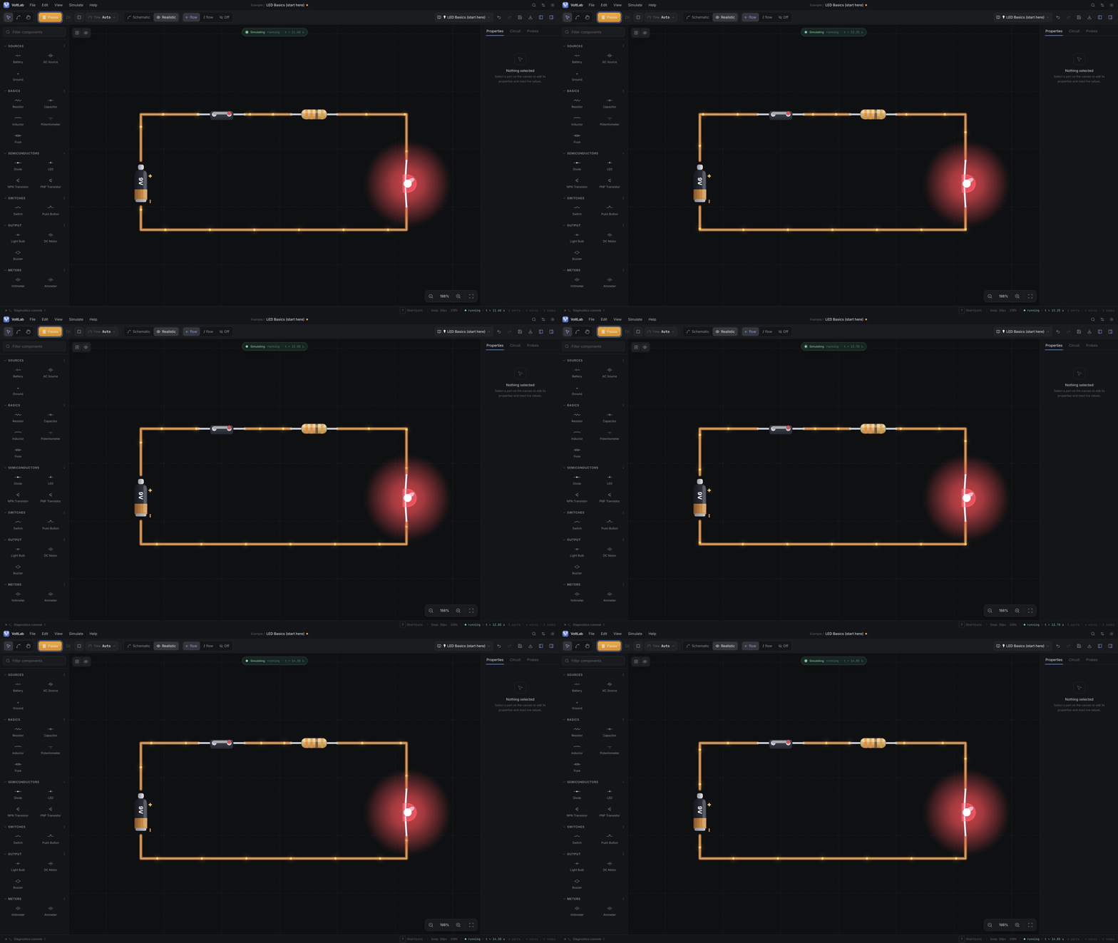
The LED Basics circuit is a small closed loop where the solver’s result is easy to see: the LED turns on, the flow overlay becomes active, and the inspector can report the live electrical values.
The LED example is close to steady state. The RC example makes the time model more visible. The capacitor remembers its previous voltage, and each transient step uses that history to calculate the next one.
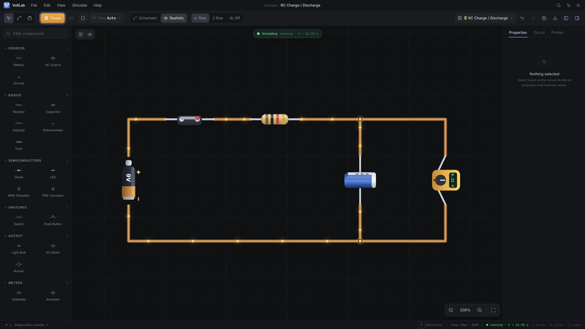
The running RC circuit shows the part of VoltLab that a static circuit diagram cannot: values changing over time as the capacitor charges and discharges.
Failure is part of the lesson
The failure lab contains deliberately problematic circuits so the product can explain its own limits.
- Floating resistor or singular island
- Shorted battery
- Conflicting voltage sources
- Valid circuit with a floating island
- Valid circuit with a shorted island
- Extreme source value
Solver decision. A failed circuit should produce something a learner can inspect. VoltLab validates the graph, identifies the failure, and reports the blocked or partial result instead of collapsing into an unexplained number.
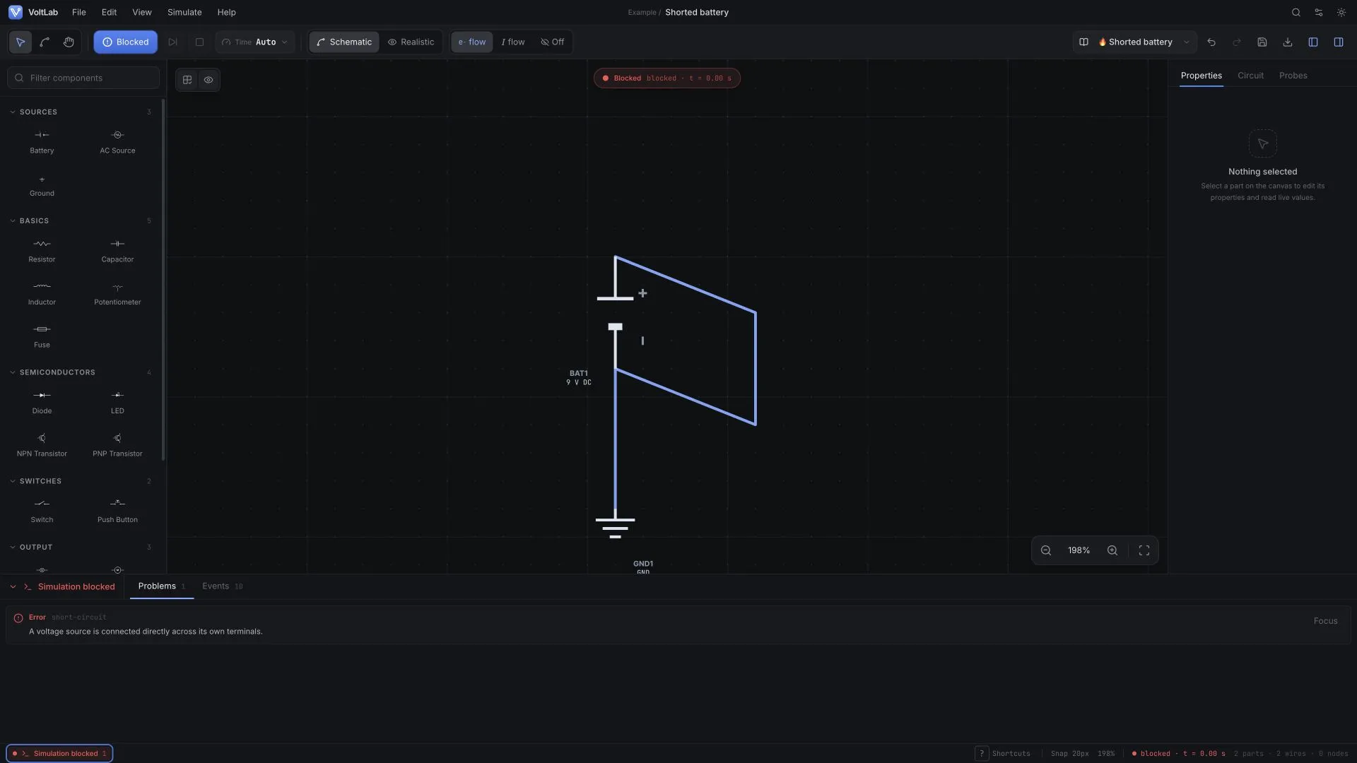
The failure-lab view pairs the circuit with a concrete explanation: the voltage source is connected directly across its own terminals.
Screenshots
The images above explain the running simulator and its failure path. This section collects the remaining views that show how the workspace changes across modes, examples, and supporting tools.
Schematic and realistic views
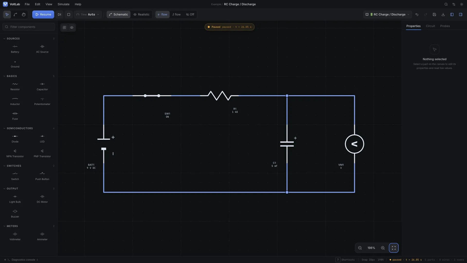
Schematic view makes the circuit topology and component labels easy to inspect.
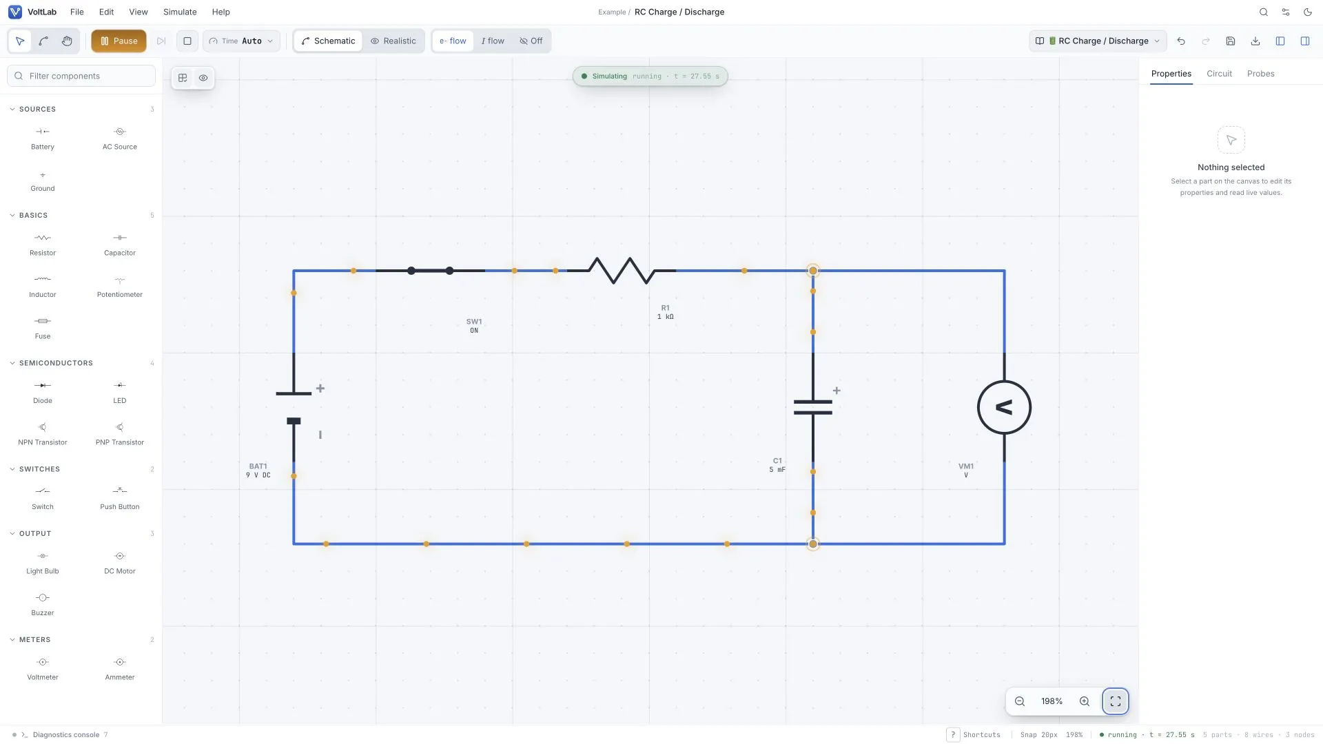
The same workspace in light mode while the simulation is running.
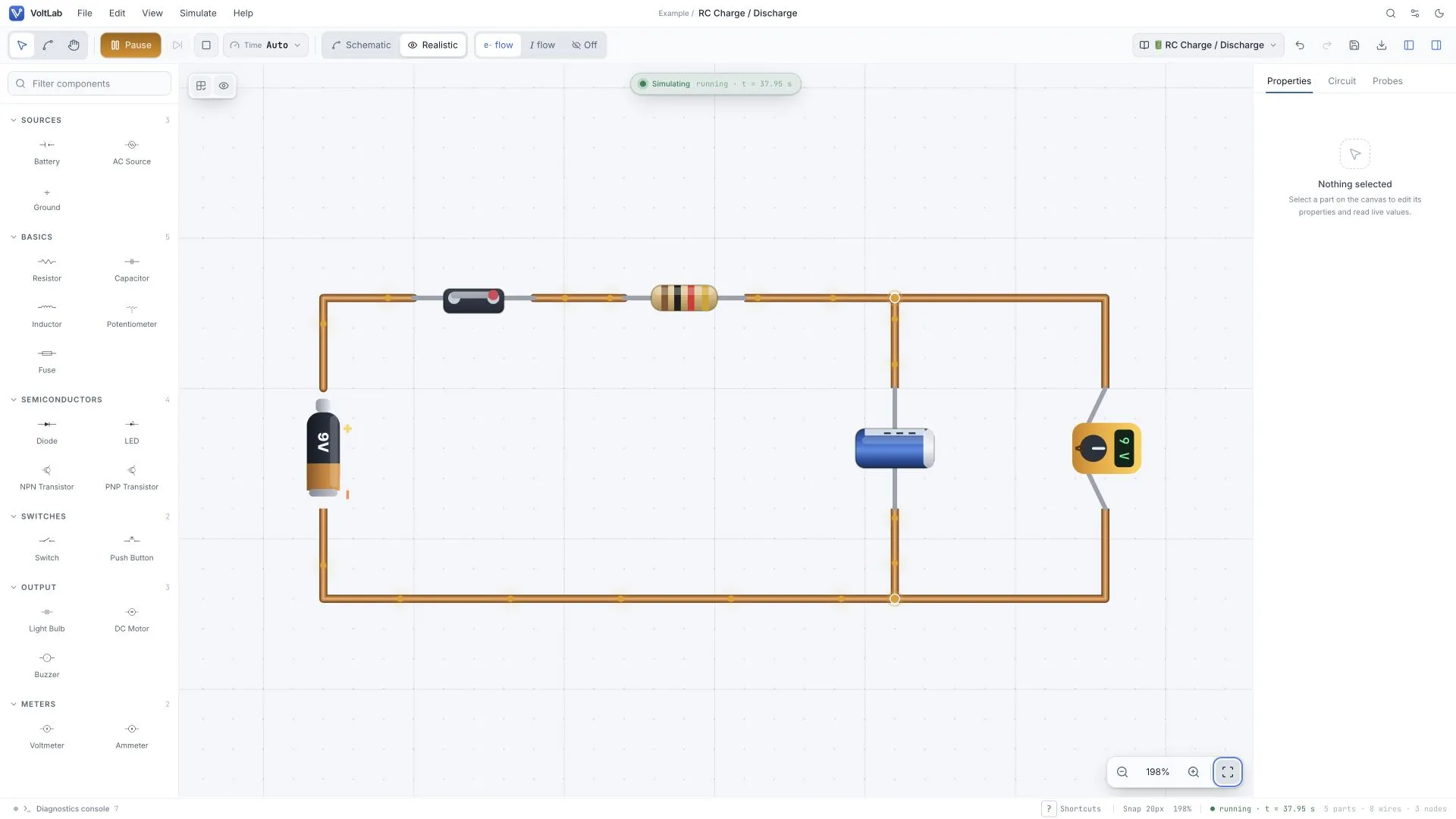
Realistic presentation in light mode, with the running state and component values still visible.
A fitted rectifier example
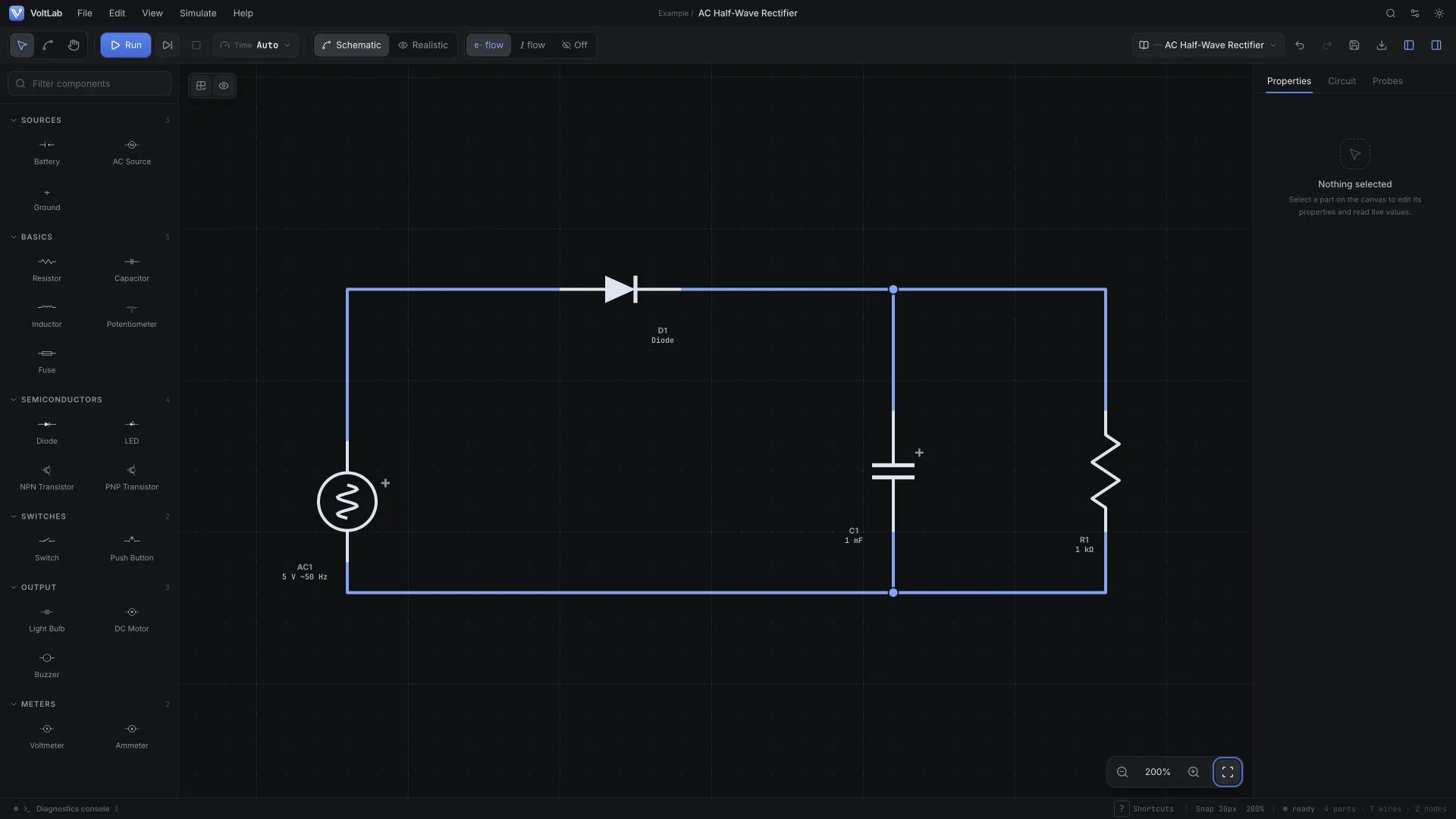
The built-in AC Half-Wave Rectifier example with the complete circuit fitted to the canvas in schematic view.
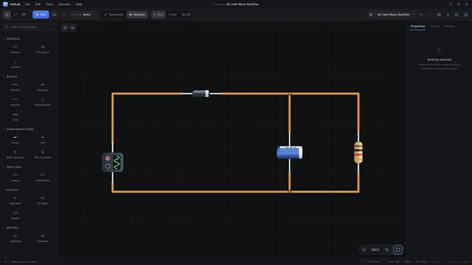
The same rectifier in realistic view, with the source, diode, capacitor, and resistor all visible.
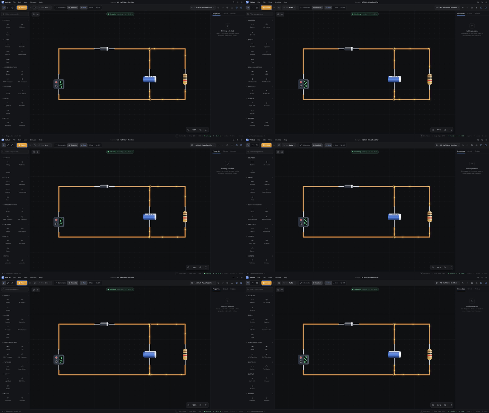
The rectifier running with the electron-flow overlay active.
The component reference
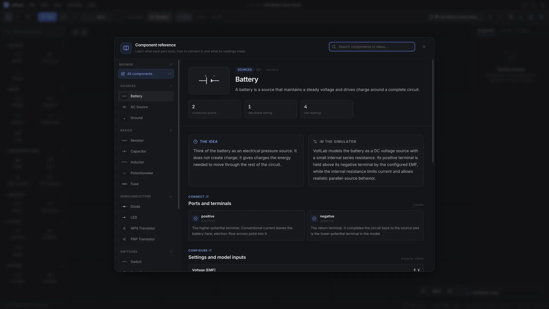
Help → Component reference opens a searchable catalogue with connection points, model inputs, live readings, explanations, and guided examples.
Another running example
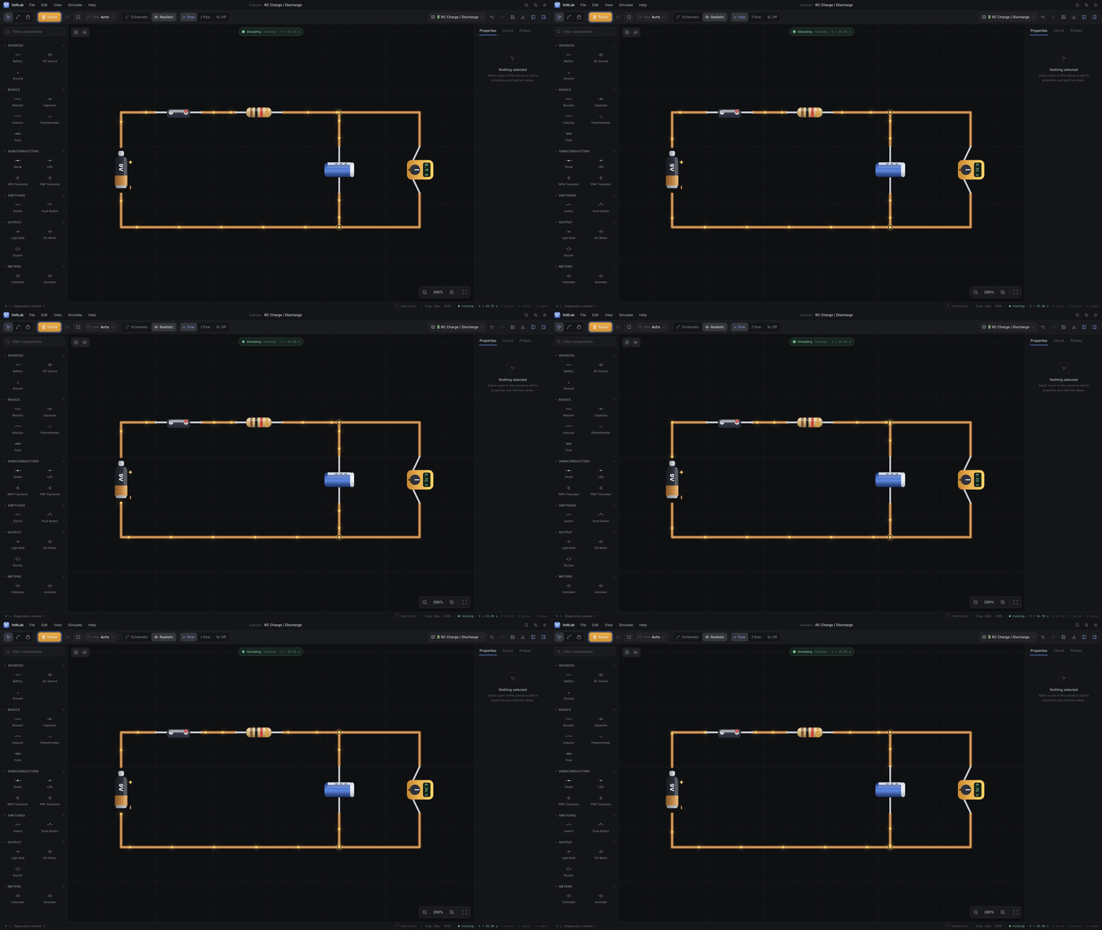
The RC Charge / Discharge example running with its realistic circuit, live meter, flow overlay, and simulation controls in view.
The code follows the same separation
| Layer | Responsibility |
|---|---|
| Domain | Circuit graph, component modules, document validation, formatting, and solver behavior |
| Application | Editing, selection, clipboard actions, history, persistence, simulation, and feedback |
| Infrastructure | Browser storage, file handling, clipboard, audio, and canvas adapters |
| Presentation | Vue controls, commands, settings, Konva rendering, wire interaction, and flow overlays |
The domain and application layers do not depend on Vue, Konva, or browser APIs. That keeps the electrical model separate from the current editor and its canvas renderer.